7 Minutes to Pywaterflood

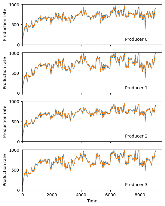
Here we will install pywaterflood, load a small (synthetic) waterflood’s production and injection data, then perform CRM to estimate the connectivities, predict production, and compare the predictions to historical production

To install pywaterflood, run

pip install pywaterflood

on the command line.

import pandas as pd
import matplotlib.pyplot as plt
from pywaterflood import CRM
import os

Waterflood history matching

First, we pull production from 4 wells and injection from 5 wells over a 298 timestep period, then we create a CRM instance where the time constants are for injector-producer pairs (per-pair) and connectivity constants are limited to 1 for each injector-producer pair. Next, we fit and predict historical production.

gh_url = "https://raw.githubusercontent.com/frank1010111/pywaterflood/master/testing/data/"
prod = pd.read_csv(gh_url + "production.csv", header=None)
inj = pd.read_csv(gh_url + "injection.csv", header=None)
time = pd.read_csv(gh_url + "time.csv", header=None)

num_threads = min(os.cpu_count(), prod.shape[1])

crm = CRM(tau_selection="per-pair", constraints="up-to one")
crm.fit(prod.values, inj.values, time.values[:, 0], num_cores=num_threads)
q_hat = crm.predict()

fig, axes = plt.subplots(len(prod.columns), figsize=(6, 8), sharex=True, sharey=True)
for i, p in enumerate(prod):
    axes[i].plot(time, prod[p], label="Production")
    axes[i].plot(time, q_hat[:, i], ls="--", label="Prediction")
    axes[i].set(xlim=(0, None), ylim=(0, None), ylabel="Production rate")
    axes[i].annotate(f"Producer {p}", xy=(7000, 100))
axes[i].set(xlabel="Time")

[Text(0.5, 0, 'Time')]

Look at inter-well connectivity

Let’s make a table of the connectivity and highlight the most important injector for each producer.

connectivity = pd.DataFrame(
    crm.gains,
    index=prod.columns.rename("Producer"),
    columns=inj.columns.rename("Injector"),
)
connectivity.T.style.highlight_max().format("{:.2}")

Producer	0	1	2	3
Injector
0	0.32	0.33	0.18	0.17
1	0.33	0.18	0.33	0.17
2	0.25	0.24	0.25	0.25
3	0.17	0.33	0.17	0.33
4	0.18	0.17	0.33	0.33

Perform pressure-compensated CRM

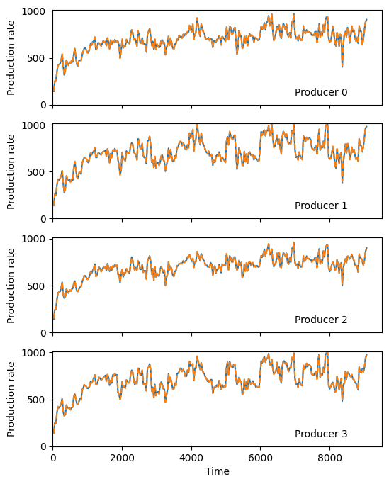
In some cases, you will have reliable pressure data for the producers in your waterflood. This is useful additional data that can improve the capacitance resistance model predictions. The approach was established by Yousef et al. (2006) and improved by Kaviani et al. (2012).

from pywaterflood import CrmCompensated

crm_p = CrmCompensated(tau_selection="per-pair", constraints="up-to one")
pressure = (1000 - prod * 0.1).values  # allow us to make something up
crm_p.fit(prod.values, pressure, inj.values, time.values[:, 0], num_cores=num_threads)
q_hat_p = crm_p.predict()

fig, axes = plt.subplots(len(prod.columns), figsize=(6, 8), sharex=True, sharey=True)
for i, p in enumerate(prod):
    axes[i].plot(time, prod[p], label="Production")
    axes[i].plot(time, q_hat_p[:, i], ls="--", label="Prediction")
    axes[i].set(xlim=(0, None), ylim=(0, None), ylabel="Production rate")
    axes[i].annotate(f"Producer {p}", xy=(7000, 100))
axes[i].set(xlabel="Time")

[Text(0.5, 0, 'Time')]