Using Buckley-Leverett

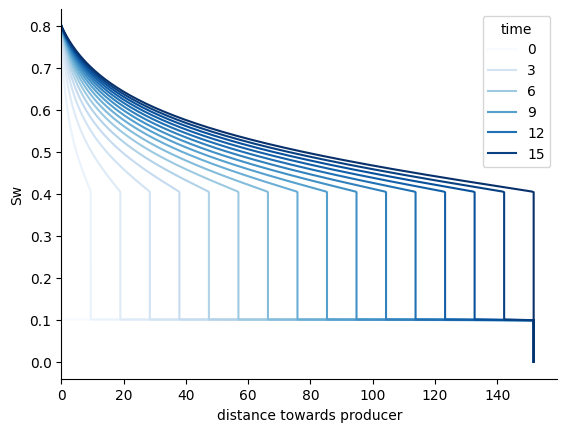
Buckley-Leverett concerns the saturation profiles in a waterflood going from the injector to the producer

The relative permeabilities here come from Brooks and Corey

import numpy as np
import matplotlib.pyplot as plt
import seaborn as sns
import pandas as pd

from pywaterflood.buckleyleverett import Reservoir, water_front_velocity, breakthrough_sw

Now, let’s set the reservoir’s rock and fluid properties

reservoir = Reservoir(
    phi=0.25,
    viscosity_oil=4.2e-3,
    viscosity_water=1e-3,
    sat_oil_r=0.2,
    sat_water_c=0.1,
    sat_gas_c=0.05,
    n_oil=2,
    n_water=2,
    flow_cross_section=1,
)

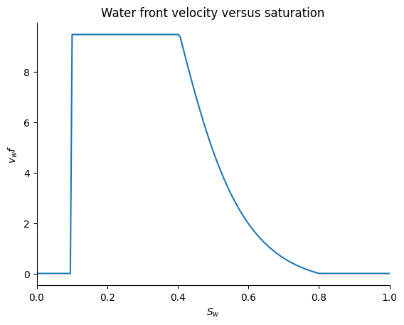
What’s the water front’s water saturation? What does the front velocity look like?

print(f"The saturation at the waterfront is {breakthrough_sw(reservoir)}")

saturations_water = np.linspace(0, 1, 200)
v_waterfront = [water_front_velocity(reservoir, s_w, 1.0) for s_w in saturations_water]

fig, ax = plt.subplots()
ax.plot(saturations_water, v_waterfront)
ax.set(
    xlim=(0, 1), xlabel="$S_w$", ylabel="$v_wf$", title="Water front velocity versus saturation"
)
sns.despine()

The saturation at the waterfront is 0.405

Okay, now how do the water flood fronts look like over time?

s_w_fronts = np.linspace(0, 1 - reservoir.sat_oil_r, 500)
df_swt = pd.DataFrame(
    {
        "time": 0.0,
        "Sw": s_w_fronts,
        "x_front": 0.0,
    }
)
front_velocities = np.array([water_front_velocity(reservoir, s_w, 1.0) for s_w in s_w_fronts])
dt = 1
end_t = 16
times = np.arange(0, end_t + dt, dt)
df_swt = pd.concat(
    [pd.DataFrame({"time": t, "Sw": s_w_fronts, "x_front": front_velocities * t}) for t in times]
)
distance_to_producer = max(df_swt["x_front"])
df_swt.loc[lambda x: x.Sw <= reservoir.sat_water_c, "x_front"] = distance_to_producer
g = sns.lineplot(df_swt, x="x_front", y="Sw", hue="time", orient="y", palette="Blues")
g.set(xlim=(0, None), xlabel="distance towards producer")
sns.despine()