Choosing your CRM

There are several different CRM models. pywaterflood offers options for capacitance resistance modeling at different levels of sophistication and robustness. Depending on the amount and quality of the data, the best model could be the full CRMIP or even a multi-layered CRMIP model, or it could be the simpler CRMP model.

import pandas as pd
import matplotlib.pyplot as plt
from pywaterflood import CRM

Data exploration

In order to decide which model, first look at the size and quantity of the data.

gh_url = "https://raw.githubusercontent.com/frank1010111/pywaterflood/master/testing/data/"
prod = pd.read_csv(gh_url + "production.csv", header=None)
inj = pd.read_csv(gh_url + "injection.csv", header=None)
time = pd.read_csv(gh_url + "time.csv", header=None)

Because this is test data, and test data can be anything, it’s measured in reservoir barrels! Nice! Otherwise, you might have to convert the oil and water produced from stock tank barrels to reservoir barrels.

Our example is a tiny field with 4 producers, 5 injectors, and 300 months of production history.

fig, (ax1, ax2) = plt.subplots(1, 2, figsize=(8, 4))
prod.join(time.rename(columns={0: "Time"})).set_index("Time").rename_axis(columns="Producer").plot(
    ax=ax1
)
inj.join(time.rename(columns={0: "Time"})).set_index("Time").rename_axis(columns="Injector").plot(
    ax=ax2
)
ax1.set(ylim=(0, None), ylabel="Production (rb)", title="Producers")
ax2.set(ylim=(0, None), ylabel="Injection (rb)", title="Injectors")
fig.tight_layout()

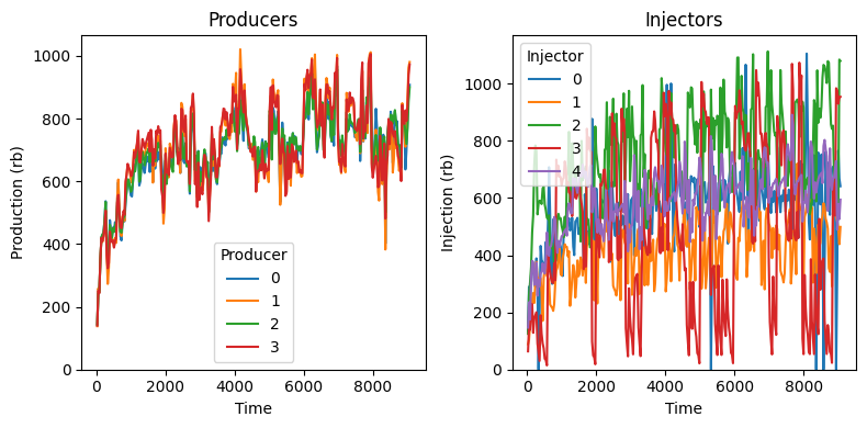
A few things jump out:

1. Clearly we’re at the start of the waterflood. Production starts very low and increases. Injection starts with injector 1 going at full throttle, and within the first year the others start catching up. This means that the CRM does not have to include primary production.

2. The injectors have high variance in injectivity, and they don’t all fluctuate in phase. This means CRM might work well! Yay!

3. There is enough data here for per-pair taus.

One more thing to check: the material balance. Why does that matter?

1. If the production is much more than the injection, you might have an aquifer. The solution for an aquifer is add a pseudo-well using either the imbalance or an aquifer influx model.

2. If the production is much less or about the same, you can apply stronger constraints to the gain constraints.

fig, ax = plt.subplots(figsize=(6, 4))
ax.plot(time, prod.sum(axis=1), label="Production")
ax.plot(time, inj.sum(axis=1), "--", label="Injection")
ax.set(xlabel="Time", ylabel="Reservoir barrels", ylim=(0, None))
ax.legend()

<matplotlib.legend.Legend at 0x7f1f2877d5d0>

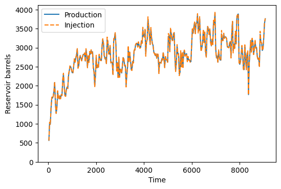
The production and injection are exactly in sync! This is very rare in real datasets, but we’re lucky.

Testing out CRMs

Now, let’s try out our first CRM. As suggested in the API docs, setting tau_selection to per-pair should almost always be the first choice. This is called the CRMIP model, and the papers tend to agree that it leads to the highest accuracy.

crm = CRM(primary=False, tau_selection="per-pair", constraints="up-to one")
crm.fit(prod.values, inj.values, time.values[:, 0])
q_hat = crm.predict()

fig, axes = plt.subplots(len(prod.columns), figsize=(6, 8), sharex=True, sharey=True)
for i, p in enumerate(prod):
    axes[i].plot(time, prod[p], label="Production")
    axes[i].plot(time, q_hat[:, i], ls="--", label="Prediction")
    axes[i].set(xlim=(0, None), ylim=(0, None), ylabel="Production rate")
    axes[i].annotate(f"Producer {p}", xy=(7000, 100))
axes[i].set(xlabel="Time")

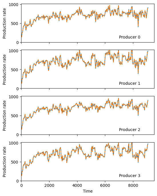
That’s a nice set of fits. Now there’s no sense in not trying out other models. What models are there to choose from? de Holanda et al catalog several other CRM models:

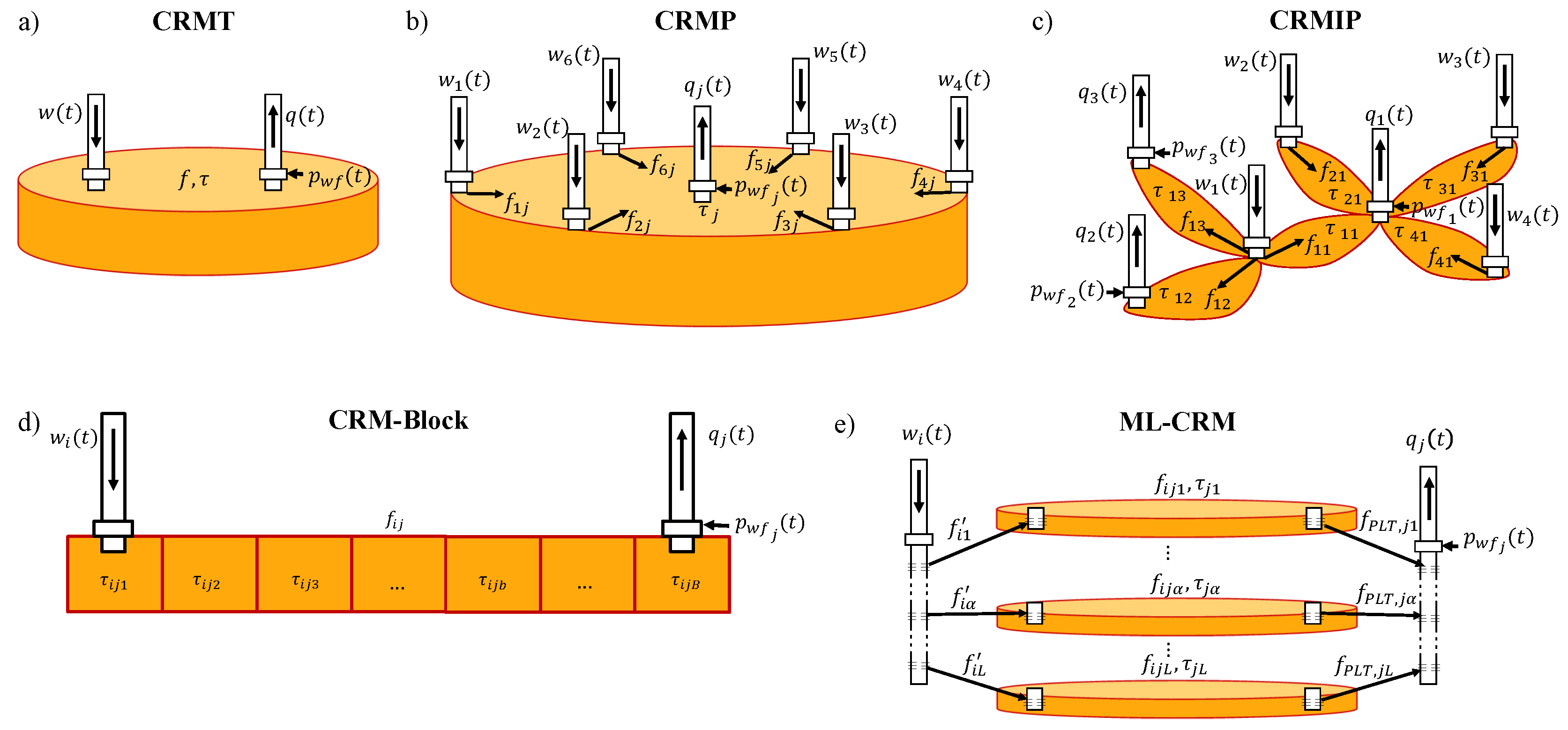
Source: A State-of-the-Art Literature Review on Capacitance Resistance Models for Reservoir Characterization and Performance Forecasting by Rafael Wanderley de Holanda, et al. (2018).

At this point, we’ve tried (and wildly succeeded with CRMIP), but let’s try some others. CRMT can be run through summing the production and injection data:

crm = CRM(primary=False, tau_selection="per-pair", constraints="up-to one")
crm.fit(prod.sum(axis=1).to_frame().values, inj.sum(axis=1).to_frame().values, time.values[:, 0])
q_hat = crm.predict()

fig, ax = plt.subplots(figsize=(6, 4))
ax.plot(time, prod.sum(axis=1), label="Production")
ax.plot(time, q_hat[:, 0], "--", label="Prediction")
ax.legend(loc="lower right")
ax.set(xlim=(0, None), ylim=(0, None), xlabel="Time", ylabel="Field-wide rb")

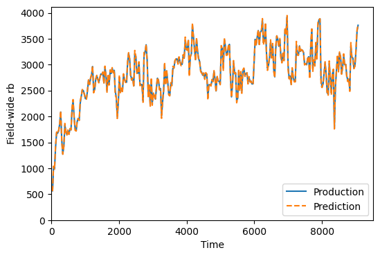
I’m not sure how useful this tank model is, but it matches production well.

In between CRMIP and CRMT in complexity is CRMP. With CRMP, you assign only one time constant for each producer, but keep estimating connectivity between each producer-injector well pair.

crm = CRM(primary=False, tau_selection="per-producer", constraints="up-to one")
crm.fit(prod.values, inj.values, time.values[:, 0])
q_hat = crm.predict()

fig, axes = plt.subplots(len(prod.columns), figsize=(6, 8), sharex=True, sharey=True)
for i, p in enumerate(prod):
    axes[i].plot(time, prod[p], label="Production")
    axes[i].plot(time, q_hat[:, i], ls="--", label="Prediction")
    axes[i].set(xlim=(0, None), ylim=(0, None), ylabel="Production rate")
    axes[i].annotate(f"Producer {p}", xy=(7000, 100))
axes[i].set(xlabel="Time")

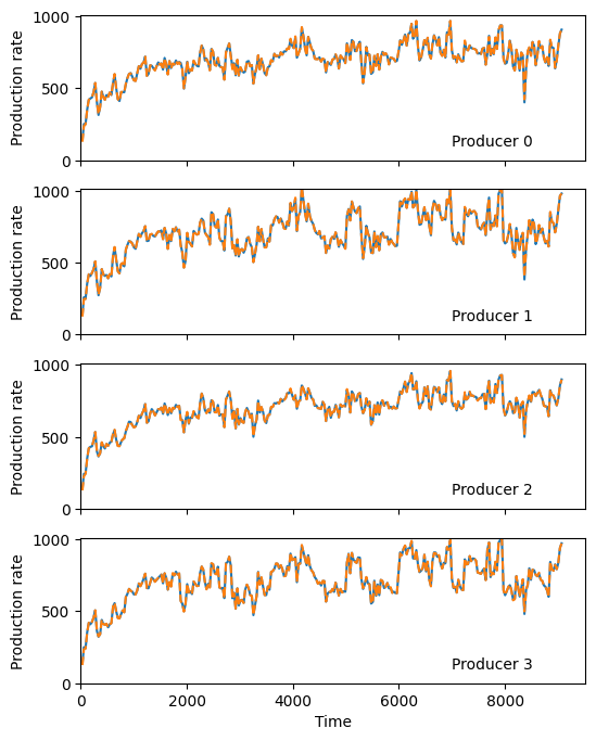
CRMP is much faster to fit than full CRMIP, but in many cases it is less accurate. In our synthetic reservoir, it seems to be doing quite well.

Two other models are also found in the literature. CRM-Block is not yet implemented in pywaterflood, but it breaks the tank models between injectors and producers into blocks. This allows for production responses to injectors to be delayed. ML-CRM is the same as CRMIP, except it relies on production and injection data being allocated to each perforation interval. With per-perforation flow information, reservoir sub-units can be studied.